 Time-history Seismic Analysis of a 5 Story Steel Building
 Time-history Seismic Analysis of a 5 Story Steel Building
[ Five Story Steel Building ]
[ Earthquake Accelerogram ]
[ Combined Modal/Newmark Analysis ]
[ Displacements ]
[ Energy Computation ]
[ Input and Output Files ]
In this example we use a combination of modal analysis and Newmark analysis to compute the linear time-history response of a steel building structure subject to earthquake ground motion loads.
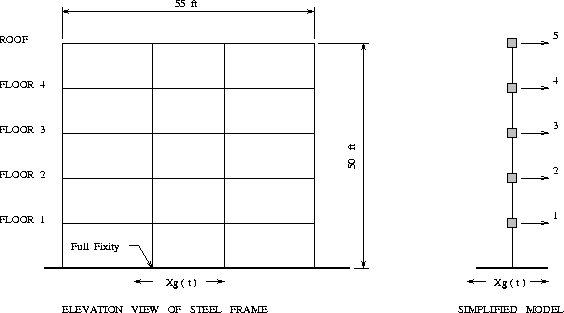
The left-hand side of Figure 1 is a simplified elevation view of the five story steel frame used in the static finite element analysis .

In contrast to the static finite element analysis problem, here we will assume that:
It follows from these two assumptions that each floor will move as a rigid body in the horizontal direction, and that the global frame behavior may be described with only five degrees of freedom. The right-hand side of Figure 1 shows the simplified model that will be used in the earthquake time-history analysis -- the shaded filled boxes represent the lumped masses at each floor level, and the global degrees of freedom begin at the first floor level and increase to the roof.
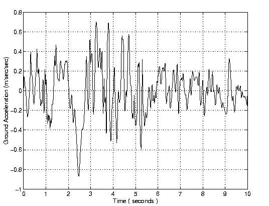
Figure 2 shows details of a 10 segment accelerograph extracted from the 1979 El Centro Earthquake ground motion.

The peak ground acceleration is 86.63 cm/sec/sec. The ground motion will be scaled so that the peak ground acceleration is 0.15 g.
The earthquake accelerogram
   /* [n] : Define earthquake loadings... */

   Elcentro = ColumnUnits( [
     14.56;    13.77;     6.13;     3.73;     1.32;    -6.81;

     ...... details of earthquake removed .....

    -10.05;   -12.35;   -15.72;     0.00  ], [cm/sec/sec] );

   ground_motion_scale_factor = 0.15*981.0/86.63;
is defined in a column matrix having units of cm/sec/sec.
Our algorithm for computing the time-history response is composed of two parts.
Part 1 -- Modal Analysis : Instead of computing the time-history response directly on the large set of coupled finite equations, we simplify the analysis by computing the eigenvalues/vectors for the steel frame, and then computing the generalized mass and stiffness matrices for the first two modes of vibration.
The essential details of ALADDIN code are:
   /* [j] : Compute and print eigenvalues and eigenvectors */

   no_eigen = 2;
   eigen       = Eigen(stiff, mass, [ no_eigen ]);
   eigenvalue  = Eigenvalue(eigen);
   eigenvector = Eigenvector(eigen);

   for(i = 1; i <= no_eigen; i = i + 1) {
       print "Mode", i ," : w^2 = ", eigenvalue[i][1];
       print " : T = ", 2*PI/sqrt(eigenvalue[i][1]) ,"\n";
   }

   PrintMatrix(eigenvector);

   /* [k] : Generalized mass and stiffness matrices */

   EigenTrans = Trans(eigenvector);
   Mstar   = EigenTrans*mass*eigenvector;
   Kstar   = EigenTrans*stiff*eigenvector;

   /* [m] : Setup Rayleigh Damping for the Framed Structure */

   rdamping = 0.05;
   W1 = sqrt ( eigenvalue[1][1]);
   W2 = sqrt ( eigenvalue[2][1]);

   A0 = 2*rdamping*W1*W2/(W1 + W2);
   A1 = 2*rdamping/(W1 + W2);

   Cstar = A0*Mstar + A1*Kstar;
Points to note are:
Part 2 -- Newmark Analysis : Newmark Analysis is conducted on the first two modes of decoupled equations. The essential details of ALADDIN code for the Newmark algorithm are:
   /* [o] : Initialize system displacement, velocity, and load vectors */

   displ  = ColumnUnits( Matrix([5,1]), [m]    );
   vel    = ColumnUnits( Matrix([5,1]), [m/sec]);
   eload  = ColumnUnits( Matrix([5,1]), [kN]);
   r      = One([5,1]);

   /* [p] : Initialize modal displacement, velocity, and acc'n vectors */

   Mdispl  = ColumnUnits( Matrix([ no_eigen,1 ]), [m]    );
   Mvel    = ColumnUnits( Matrix([ no_eigen,1 ]), [m/sec]);
   Maccel  = ColumnUnits( Matrix([ no_eigen,1 ]), [m/sec/sec]);

   /*
    * [q] : Allocate Matrix to store five response parameters --
    *       Col 1 = time (sec);
    *       Col 2 = 1st mode displacement (cm);
    *       Col 3 = 2nd mode displacement (cm);
    *       Col 4 = 1st + 2nd mode displacement (cm);
    *       Col 5 = Total energy (Joules)
    */

   dt     = 0.02 sec;
   nsteps = 600;
   beta   = 0.25;
   gamma  = 0.5;

   response = ColumnUnits( Matrix([nsteps+1,5]), [sec], [1]);
   response = ColumnUnits( response,  [cm], [2]);
   response = ColumnUnits( response,  [cm], [3]);
   response = ColumnUnits( response,  [cm], [4]);
   response = ColumnUnits( response, [Jou], [5]);

   /* [r] : Compute (and compute LU decomposition) effective mass */

   MASS  = Mstar + rdamping*dt*Cstar + Kstar*beta*dt*dt;
   lu    = Decompose(Copy(MASS));

   /* [s] : Mode-Displacement Solution for Response of Undamped MDOF System  */

   MassTemp = -mass*r;
   for(i = 1; i <= nsteps; i = i + 1) {
       if(i == 2) {
          SetUnitsOff;
       }

    /* [s.1] : Update external load */

       if(i <= 500) then {
          eload = MassTemp*Elcentro[i][1]*ground_motion_scale_factor;
       } else {
          eload = MassTemp*(0)*ground_motion_scale_factor;
       }

       Pstar = EigenTrans*eload;

       R = Pstar - Kstar*(Mdispl + Mvel*dt + Maccel*(dt*dt/2.0)*(1-2*beta)) -
           Cstar*(Mvel + Maccel*dt*(1-gamma));

    /* [s.2] : Compute new acceleration, velocity and displacement  */

       Maccel_new = Substitution(lu,R);
       Mvel_new   = Mvel   + dt*(Maccel*(1.0-gamma) + gamma*Maccel_new);
       Mdispl_new = Mdispl + dt*Mvel + ((1 - 2*beta)*Maccel +
                    2*beta*Maccel_new)*dt*dt/2;

    /* [s.3] : Update and print new response */

       Maccel = Maccel_new;
       Mvel   = Mvel_new;
       Mdispl = Mdispl_new;

    /* [s.4] : Combine Modes */

       displ = eigenvector*Mdispl;
       vel   = eigenvector*Mvel;

    /* [s.5] : Compute Total System Energy */

       a1 = Trans(vel);
       a2 = Trans(displ);
       e1 = a1*mass*vel;
       e2 = a2*stiff*displ;
       energy = 0.5*(e1 + e2);

    /* [s.6] : Save components of time-history response */

       response[i+1][1] = i*dt;
       response[i+1][2] = eigenvector[1][1]*Mdispl[1][1];
       response[i+1][3] = eigenvector[1][2]*Mdispl[2][1];
       response[i+1][4] = displ[1][1];
       response[i+1][5] = energy[1][1];
   }
Points to note are:
Columns 2 through 4 of the response matrix store the mode 1, mode 2, and mode 1+2, time-history displacements.

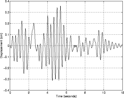
Figure 3 shows, for example, the time-history displacement of the roof for mode 1 + mode 2 when Rayleigh damping is set to 5%.
Notice that once the ground motions finishes (at t = 10 sec), the amplitude of roof displacement decreases steadily, and with a period very close to the first mode of vibration.
The script of ALADDIN code:
       a1 = Trans(vel);
       a2 = Trans(displ);
       e1 = a1*mass*vel;
       e2 = a2*stiff*displ;
       energy = 0.5*(e1 + e2);
is located inside the main loop for Newmark Integration, and computes the sum of the kinetic and potential energy at each time step.

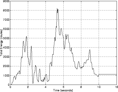
Figure 4 shows the sum of kinetic + potential energy versus time for an undamped steep frame building.
Theoretical considerations indicate that Newmark will conserve energy exactly when:
Hence, it is pleasing to see that in the interval t = 10-12 seconds, kinetic energy + potential energy is constant.