 Behavior of Lead-Rubber Isolators under Cyclic Shear Loadings
 Behavior of Lead-Rubber Isolators under Cyclic Shear Loadings
[ Problem Statement ]
[ Experimental Procedure ]
[ Finite Element Model ]
[ Hysteretic Behavior ]
[ Input/Output Files ]
You will need Aladdin 2.0 to run this problem.
Before a new type of lead-rubber bearing can be used in a large structural system, design codes require that its hysteretic force-displacement capabilities be validated by experiment. In a typical experimental procedure the bearing displacements will be measured for a pre-determined combination of axial and cyclic shear forces.
In this example we demonstrate that the FRAME_3DS finite element can replicate the cyclic shear behavior of lead-rubber bearings derived from a force-controled experiment. Analysis procedures that incorporate nonlinear finite elements of this type are an important part of performance-prediction for base-isolated structures.
Laminated Lead-Rubber Bearings
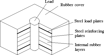
A lead-rubber bearing is a laminated rubber bearing with a lead plug down its center, as depicted in Figure 1.

The rubber/steel laminated bearing is designed to carry the weight of the structure and provide post-yield elasticity. The lead core deforms plastically under shear deformations. Its size can be selected to produce the required amount of damping.
In the design of highway bridges that must resist severe lateral loads, there are several benefits in using lead-rubber bearings for base-isolation:
The size of the lead plug is proportional to the yield strength of the isolator. The post-yielding stiffness is proportional to the rubber bearing stiffness, and increases with the plan size of the rubber bearing and reductions in the isolator height.
During severe seismic attacks, however, the lead plug is capable of deforming through many low-cycle plastic deformations without a loss of strength occuring.
Experimental studies indicate that lead responds essentially with elastic-perfectly plastic loops. Hence, for practical purposes the post-yielding isolator stiffness is equal to the stiffness of the rubber bearing alone. The global hysteresis loop is a bi-linear solid with an initial elastic stiffness
k_1 = 10 . k_r
where k_r is the stiffness of rubber, then followed by a post yield stiffness k_2 = k_r [2,3].
In this section we will briefly outline the experimental procedure for testing a single lead-rubber bearing in cyclic shear under compressive axial loads of 3125 kN.
Geometry and Material Properties
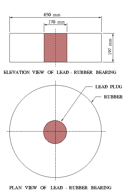
Figure 2 is a plan and elevation view of the lead-rubber laminated bearing we will consider in the analysis.

These dimensions correspond to the largest lead-rubber isolator tested in an experimental program conducted by Robinson and co-workers [2].
In Aladdin the geometry of the lead-rubber bearing is represented by the variables:
    iso_h = 197 mm;
    r_dia = 650 mm;
    l_dia = 170 mm;
The material properties of the lead are:
    Kv = 600 kN/mm;
    Ea = Kv*iso_h/(PI/4*r_dia*r_dia);

    E_lead  = Ea;
    G_lead  = 130 MPa;
    fv_lead = 10 MPa;
And the material properties of rubber are:
    Kr = 1.75 kN/mm;
    E_rubber = Ea;
    G_rubber = Kr*iso_h/(PI/4*(r_dia*r_dia-l_dia*l_dia));
Here "E_lead" and "E_rubber" are the modulus of elasticity in the isolator's axial direction. The stiffness of the lead and rubber in the lateral direction(s) are given by "G_lead" and "G_rubber," respectively. "fv_lead" represents the yield stress of lead.
Test Procedure
The following test procedure will be used to assess the force-displacement capabilities of the lead-rubber laminated bearing under combined axials loads and cyclic shear loadings:
We now consider the problem of modeling the lead-rubber isolator with the fiber element in ALADDIN. Because the lead-rubber isolator is composed of two different materials, each with its own shear modulus, the isolator behavior is modeled with a FIBER_3DS element.
Nodes and Elements
The block of code:
    AddNode( 1, [ 0 m, 0 m, iso_h ] );
    AddNode( 2, [ 0 m, 0 m,   0 m ] );

    AddElmt( 1, [1,2], "isolator_attr");
generates a finite element mesh containing two nodes a one finite element having the attribute label "isolator_attr".
After the boundary condition
FixNode( 2, [1,1,1,1,1,1] );
has been applied, the isolator finite element model has six d.o.f. See Figure 3.

Flexural Behavior
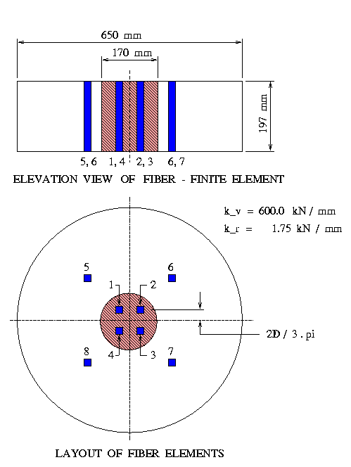
Figure 4 is a plan view of a lead-rubber isolator, showing the section dimensions and positions of the fiber elements.

We model the flexural behavior of the isolator by partitioning the lead and rubber sections into quadrants -- each quadrant of the isolator is modeled with two fibers, one for the lead, and a second for the rubber.
The fibers are positioned at the centroid of the material quadrant. The material properties are as mentioned in the previous section.
Shear Behavior
Shear deformations in the lead and rubber are modeled with springs having equivalent shear stiffness (i.e., G_lead and G_rubber), one for each fiber.

Finite Element Attributes
For simplicity the three-dimensional behavior of the base-isolation pad will be modeled with only one fiber finite element containing 8 fibers.
    ElementAttr("isolator_attr") { type     = "FIBER_3DS";
                                   section  = "iso_sec";
                                   material = "iso_mat";
                                   fiber    = "iso_fib";
                                 }
Material and Section Properties
    SectionAttr("iso_sec") { area  = PI/4*r_dia*r_dia;
                             depth = r_dia;
                             width = r_dia;
                             unit_weight  = 0.0001 kN/m;
                             shear_factor = 1.0;
                             J            = PI/32*r_dia^4;
                           }

    MaterialAttr("iso_mat") { poisson  = 0.4;
                              E        = 3.562e8 N/m^2;
                            }
Fiber Geometry
The block of code:
    no_fiber_type = 2;
    divid_no      = 4;
    theta = PI/divid_no;
    l_r = l_dia*sin(theta)/theta/3;
    r_r = r_dia*sin(theta)/theta/3;
    no_fiber = 2*divid_no;

    fcoord = Matrix([ 2, no_fiber ]);
    farea  = Matrix([ 1, no_fiber ]);
    fmap   = Matrix([ 1, no_fiber ]);
    for( i=1 ; i<=divid_no ; i=i+1 ) {
       fcoord[1][i] = l_r*cos((2*i-1)*theta);
       fcoord[2][i] = l_r*sin((2*i-1)*theta);
       farea[1][i]  = theta*l_dia*l_dia/4;
       fmap[1][i]   = 1;

       fcoord[1][i+divid_no] = r_r*cos((2*i-1)*theta);
       fcoord[2][i+divid_no] = r_r*sin((2*i-1)*theta);
       farea[1][i+divid_no]  = theta*(r_dia*r_dia - l_dia*l_dia)/4;
       fmap[1][i+divid_no]   = 2;
    }
defines three matrices, "fcoord", "farea", and "fmap" which store the coordinates, equivalent areas and material mappings for the eight fibers shown in the lower half of Figure 4.
Material Properties of Individual Fibers
The block of code:
    fattr  = Matrix([ 6, no_fiber_type ]);
    for( j=1 ; j <= no_fiber_type ; j=j+1 ) {
       if( j == 1 ) {  /* lead */
          fattr[1][j] = E_lead;
          fattr[2][j] = E_lead;
          fattr[3][j] = 10e6 MPa;
          fattr[4][j] = G_lead;
          fattr[5][j] = G_lead*1e-6;
          fattr[6][j] = fv_lead;
       }
       if( j == 2 ) {  /* rubber */
          fattr[1][j] = E_rubber;
          fattr[2][j] = E_rubber;
          fattr[3][j] = 10e6 MPa;
          fattr[4][j] = G_rubber;
          fattr[5][j] = G_rubber;
          fattr[6][j] = 10e6 MPa;
       }
    }

    FiberAttr( no_fiber, "iso_fib" ) { FiberMaterialAttr = fattr;
                                       FiberCoordinate   = fcoord;
                                       FiberArea         = farea;
                                       FiberMaterialMap  = fmap;
                                     }
allocates memory for a 6-by-2 array fattr, and initializes its contents with the material properties shown in Table 2.
| Fiber Attribute | Lead | Rubber |
| Young's Modulus | E_lead | E_rubber |
| Tangent Young's Modulus | E_lead | E_rubber |
| Yield Stress | 10e06 MPa | 10e06 MPa |
| Shear Modulus | G_lead | G_rubber |
| Tangent Shear Modulus | G_lead/1000000 | G_rubber |
| Shear Yield Stress | fv_lead | 10e06 MPa |
The test-procedure is as follows:
Apply Compressive Loading
First we apply a compressive force of 3.25 MN to the isolator:
    stiff = Stiff();
    NodeLoad( 1, [ 0 kN, 0 kN, -3150 kN, 0 kN*m, 0 kN*m, 0 kN*m] );
    P_old = ExternalLoad();
    displ = Solve( stiff, P_old );
    ElmtStateDet( displ );
    stiff = Stiff();
and compute the element state determination.
Force-Controled Shear Loading
The shear loading is applied in 180 increments, i.e.,
    if( step == 1 ) then {
           NodeLoad( 1, [ 200 kN, 0 kN, 0 kN, 0 kN*m, 0 kN*m, 0 kN*m] );
    } else {
       if( step <= 21 ) {
           NodeLoad( 1, [  10 kN, 0 kN, 0 kN, 0 kN*m, 0 kN*m, 0 kN*m] );
       }
       if( step > 21  && step <= 101 ) {
           NodeLoad( 1, [ -10 kN, 0 kN, 0 kN, 0 kN*m, 0 kN*m, 0 kN*m] );
       }
       if( step > 101 ) {
           NodeLoad( 1, [  10 kN, 0 kN, 0 kN, 0 kN*m, 0 kN*m, 0 kN*m] );
       }
    }
At each step of the analysis we compute the nonlinear displacements corresponding to the force-controlled shear loading. The Aladdin code is really quite straight forward:
   no_step = 180;
   for( step=1 ; step <= no_step+1 ; step=step+1 ) {

      /* Force-controled shear load increment */

         ..... details shown above ....

      /* Compute external loads */

      P_new = ExternalLoad();
      dP    = P_new - P_old;
      P_old = P_new;

      /* Newton-Raphson Iteration for State Determination */

      while( L2Norm(dP) > 0.001 ) {

         dp    = Solve( stiff, dP );
         displ = displ + dp;

         ElmtStateDet( dp );

         stiff = Stiff();
         PR    = InternalLoad( displ );
         dP    = P_new - PR;        /* Compute unbalanced force */
      }

      UpdateResponse();
      print step,"\t",P_new[max_dof][1](kN),"\t",displ[max_dof][1](mm),"\n";
   }
Comparison of Finite Element and Experimental Behavior
Figure 6 compares the force-displacement relationship for the FIBER_3DS element with the experimental data generated by Robinson [2].

Since there is a good match between these curves, we conclude that the bi-linear fiber element will provide sufficient modeling accuracy for this study.
References